Greenhouse Climate Modeling with ASHRAE and Python

Greenhouse climate control is a heating, ventilation, and air conditioning (HVAC) problem first, a controls problem second, and a crop problem after that. If the enclosure math is wrong, no amount of controller tuning will rescue the system. You will size fans incorrectly, overestimate heating capacity, and spend summer afternoons wondering why the room still runs hot.

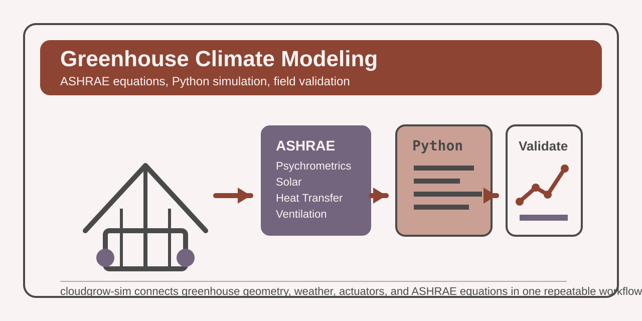
That is why I find cloudgrow-sim interesting. It does not begin with dashboards or farm-tech marketing language. It begins with American Society of Heating, Refrigerating and Air-Conditioning Engineers (ASHRAE) Handbook-Fundamentals equations for psychrometrics, solar radiation, heat transfer, and ventilation, then carries those equations into a Python simulation engine you can drive from YAML.

The interesting part is not that the package simulates a greenhouse. Many tools can produce a temperature trace. The interesting part is that the model is explicit about where each layer comes from, what it calculates, and how you can validate it. That makes it useful for design work instead of presentation work.

Greenhouse Climate Is Coupled Physics

A greenhouse is not a single temperature control loop. It is several coupled energy and moisture loops that push against each other all day.

Solar load enters through the covering and changes with latitude, season, cloud cover, and roof geometry. Conduction moves heat through the glazing and structure whenever indoor and outdoor conditions diverge. Ventilation removes sensible heat, but it also changes humidity and carbon dioxide concentration. Evaporative cooling helps in hot dry weather, then loses value as outside air approaches saturation.

That coupling is why rule-of-thumb sizing breaks down quickly. A fan that looks adequate on a static cubic-feet-per-minute chart may still underperform once solar gain, infiltration, thermal mass, and humidity control interact. The model has to solve the whole system, not just a single load path.

cloudgrow-sim organizes that problem into four physics blocks that map cleanly to the ASHRAE handbook chapters called out in the code and user guide.

Layer	Source	What it computes	Example check
Psychrometrics	Chapter 1	saturation pressure, humidity ratio, wet-bulb, dew point, enthalpy, density	20 C at 50% relative humidity (RH) gives humidity ratio around 0.0073 kg/kg
Solar	Chapter 14	solar position, irradiance, diffuse radiation, photosynthetically active radiation (PAR) conversion	1000 W/m^2 solar converts to about 2057 umol/m^2/s photosynthetically active radiation (PAR)
Heat transfer	Chapters 4, 25, 26	conduction, convection, radiation, sky temperature, surface balance	U=5, A=100, dT=15 yields 7500 W conductive loss
Ventilation	Chapter 26	infiltration, stack flow, wind-driven flow, sensible and latent exchange	1000 m^3 at 0.5 air changes per hour (ACH) yields about 0.139 m^3/s airflow

Those checks are not hand-wavy examples. They are the same order of magnitude asserted in the project test suite. The psychrometric tests also cross-check several values against CoolProp, which is exactly the kind of independent reference I want before trusting any moist-air implementation.

What the ASHRAE Mapping Looks Like in Code

The clearest signal in the repository is the psychrometrics module. It cites ASHRAE Handbook-Fundamentals 2021, Chapter 1 directly in the module docstring and implements the Hyland-Wexler saturation pressure correlation, humidity ratio, wet-bulb iteration, dew point, enthalpy, and moist-air density functions.

That matters because greenhouse humidity control goes wrong fast when the moist-air math is approximate. Relative humidity alone is not enough. You need humidity ratio and enthalpy if you want to reason correctly about ventilation, evaporation, and latent load.

The ventilation module follows the same pattern. It references Chapter 26 and separates the problem into infiltration, stack effect, wind-driven flow, combined natural ventilation, mechanical fan flow, and sensible versus latent exchange. That is exactly how I would want to reason about a real enclosure. A vent does not just move air. It moves heat and moisture, and the balance changes with outside conditions.

The solar and heat-transfer modules complete the loop. Solar position and irradiance determine the gain term. Conduction, convection, radiation, sky temperature, and ground temperature determine loss and exchange terms. Once those pieces exist, the simulation engine can update the greenhouse state step by step instead of relying on a single static balance point.

That is the difference between a calculator and a model. A calculator answers one question. A model lets you replay the day.

From Physics to a Runnable Scenario

One of the better design choices in cloudgrow-sim is that the physics do not force you into Python-first workflow. You can define a scenario declaratively in YAML, validate it, and run it from the CLI.

This is a trimmed version of the style the project uses for full-climate scenarios:

name: "Validation Greenhouse"
time_step: 60.0
duration: 86400.0

location:
  latitude: 37.5
  longitude: -77.4
  elevation: 50.0
  timezone: "America/New_York"

geometry:
  type: gable
  length: 30.0
  width: 10.0
  height_ridge: 5.0
  height_eave: 3.0

covering:
  material: double_polyethylene

components:
  sensors:
    - type: temp_humidity
      name: dht_interior
      location: interior

    - type: solar_radiation
      name: pyranometer
      location: exterior

  actuators:
    - type: exhaust_fan
      name: exhaust_1
      controller: cooling_pid
      max_flow_rate: 5.0
      power_consumption: 500.0

    - type: evaporative_pad
      name: evap_pad
      controller: evap_control
      pad_area: 6.0
      saturation_efficiency: 0.85

  controllers:
    - type: pid
      name: cooling_pid
      process_variable: dht_interior.temperature
      setpoint: 26.0
      kp: 0.5
      ki: 0.1
      kd: 0.05
      output_limits: [0.0, 1.0]
      reverse_acting: true

    - type: hysteresis
      name: evap_control
      process_variable: dht_interior.temperature
      setpoint: 30.0
      hysteresis: 2.0
      reverse_acting: true

weather:
  source: csv
  file: "weather/richmond-july.csv"

Then run it with the CLI:

cgsim validate validation-greenhouse.yaml
cgsim run validation-greenhouse.yaml --format json --output-dir ./results

That structure matters for practical work. Growers, integrators, and controls engineers often want to change geometry, covering material, or actuator sizing without editing source code. YAML is the correct abstraction for that layer.

Validation Should Happen in Three Stages

The phrase “real-world validation” gets abused in simulation discussions. A lot of people mean “the graph looked plausible.” That is not validation. Plausibility is the first filter, not the last one.

I would validate a greenhouse model in three stages.

1. Equation-level validation

This is the floor. If saturation pressure, humidity ratio, air density, or ventilation flow are wrong, every downstream result is wrong.

The repository already does useful work here. The psychrometric test suite checks values like saturation pressure at 0 C and 20 C, dew point round-trips, wet-bulb behavior, and enthalpy ranges. Where CoolProp is available, the tests compare ASHRAE results against CoolProp.HumidAirProp and require relative error under 1 percent for selected temperatures.

That is the right starting point. Before you calibrate to a greenhouse, calibrate to physics references.

2. Scenario-level validation

This is where you check whether the whole system behaves like a greenhouse instead of a collection of correct formulas.

The built-in scenarios are useful here because they span credible operating envelopes:

basic: Richmond, Virginia, 10 m x 6 m, one fan, one hysteresis controller
full-climate: Richmond commercial house with staged fans, evaporative pad, heater, roof vents, and thermal mass
winter-heating: Boston cold-weather stress case with 25 kW main heat plus 15 kW backup
summer-cooling: Phoenix hot-weather stress case with four high-capacity fans and 85% efficient evaporative cooling

Those scenarios let you ask the questions that matter early in design work. Does the heating case stay within realistic temperature bounds? Does the cooling case settle or oscillate? Does the controller chatter? Does changing the time step produce meaningfully different behavior? The engine test suite already guards some of that behavior with rate limits and clamped state ranges.

3. Field replay and error measurement

This is the part that turns a physics engine into an engineering tool. Synthetic weather is fine for controller shakeout. It is not enough for calibration. The model has to replay measured weather, emit telemetry, and let you compare simulated state against sensor logs.

cloudgrow-sim already supports two pieces of that workflow: CSV weather input and a state-update event bus. That is enough to build a practical validation loop.

from cloudgrow_sim.core.config import load_config
from cloudgrow_sim.core.events import EventType, get_event_bus
from cloudgrow_sim.simulation.factory import create_engine_from_config

rows = []

bus = get_event_bus()


def capture_state(event):
    rows.append(
        {
            "timestamp": event.timestamp.isoformat(),
            "interior_temperature": event.data["interior_temperature"],
            "interior_humidity": event.data["interior_humidity"],
            "solar_radiation": event.data["solar_radiation"],
        }
    )


bus.subscribe(EventType.STATE_UPDATE, capture_state)

config = load_config("validation-greenhouse.yaml").model_copy(
    update={"emit_events": True, "emit_interval": 5}
)
engine = create_engine_from_config(config)
stats = engine.run()

print(stats.steps_completed)
print(rows[:3])

With that telemetry stream, you can align simulation timestamps with logger exports and compute straightforward error metrics: mean absolute temperature error, peak midday bias, overnight recovery error, or humidity error during fan staging.

That is the workflow I would trust. Replay measured weather, export event telemetry, compare against measured indoor conditions, then change one parameter at a time: covering U-value, infiltration assumption, fan flow, thermal mass, controller gains.

What I Think This Model Can Assist With Today

I wrote cloudgrow-sim, so I do not want to oversell what it is today. I think it can already assist with enclosure and controls questions, but it still needs substantially more validation, more field replay, and more side-by-side testing before I would describe it as production-ready greenhouse tooling.

I am comfortable using it to compare covering materials, estimate whether a fan package looks undersized, study winter heating load, test hysteresis versus PID control, or quantify how much thermal mass changes nighttime recovery. I would also use it to sanity-check whether a proposed greenhouse geometry makes natural ventilation plausible before buying hardware. Those are design aids, not final answers.

I would not treat it as a crop physiology model yet. In the current public tree, the emphasis is clearly enclosure physics, weather, sensors, actuators, and controllers. I do not see crop transpiration, canopy resistance, or disease-pressure modeling in the exposed modules and docs. That is not a criticism. It is scope discipline.

That scope discipline is healthy. Too many agriculture tools promise whole-farm omniscience and deliver a pretty chart. I think a greenhouse climate simulator should first answer the questions it can answer well:

How much heat enters and leaves the enclosure?
How quickly does ventilation move the state?
What does humidity do when outside air changes?
Which controller and actuator combination actually stabilizes the room?

Once those answers are solid, you can layer crop models on top.

Why This Matters in Practice

The payoff is not academic elegance. The payoff is fewer bad decisions.

If the model tells you that your “cheap” covering increases winter heat loss enough to require another 10 kW of heater capacity, that is a purchasing decision. If the simulated summer case shows the evaporative pad only helps for a few afternoon hours before outside humidity collapses the advantage, that is a design decision. If telemetry replay shows your assumed infiltration is too low by a factor of two, that is a maintenance decision because the enclosure is leakier than the spec sheet said.

That is where standards-based simulation becomes useful on a farm. It narrows the space of guesses before you spend capital or lose a crop window.

ASHRAE is not overkill for greenhouse work. It is the correct starting point if you want the greenhouse to behave like a physical system instead of a hopeful spreadsheet.

Explore the cloudgrow-sim models if you are building greenhouse controls, comparing envelope options, or trying to make your next climate decision from measured physics instead of intuition.

Also published on Epic Pastures: Greenhouse Climate Modeling with ASHRAE and Python for farm-side readers running their own greenhouse builds.